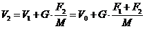
It can therefore, except for the
constant, be described as the product of a parameter Pi for the body Li,
and a parameter Qj for the
instrument Ij. And thereby
we will, via an empirical route, have found a relationship of the form (1), in
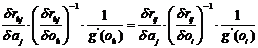
which you should then have
|
 and and 
|
(4)
|
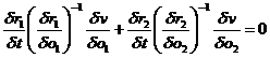
But precisely this way of writing
the parameters - that is as Qj itself, but the reciprocal value of Pi - requires an explanation
in addition to (3) and its formal paraphrase into (1). It is given in two
supplementary experiments - once again "thought experiments". From the first it
follows that if you let two instruments Ij
and Ik act immediately one
after the other on the same body Li,
the effect is the same as if it were just one instrument with the parameter
|

|
(5)
|
or according to (4)
|

|
(5a)
|
The second experiment shows that if
two bodies Lh and Li are attached together, they function
as one body when influenced by an instrument Ij, but that the parameter P(hi) for the compound body satisfies the relationship
|

|
(6)
|
that is with the notation of (4):
|

|
(6a)
|
Hereby it is first and foremost
realised that the parameters that form parts of the law (1) as "mass" and
"force" need not be individually defined, nor by each other; they can be
included simultaneously through what can be determined, i.e. the structure of the accelerations in the
thought experiment (2), in which
composite objects and instruments that act serially are included.
To this may be added that in the
additive formulas (5) and (6) for the parameters that form a part of (3), there
is a motivation for attaching the terms "mass" and "force" on  and Qj
respectively. The intuitive perception of the phenomenon "force" is not only
that the effect increases with increasing "exertion of force", but also that it
happens "quantitatively", i.e., that for example, the application of the same
force twice in a row on the same body has the same effect as the "double exertion
of force". Likewise, the intuitive perception of the phenomenon "mass" is, for
example, that two identical bodies that are tied together have the "same
inertia" - are equally difficult to move - as one body with "double the mass".
and Qj
respectively. The intuitive perception of the phenomenon "force" is not only
that the effect increases with increasing "exertion of force", but also that it
happens "quantitatively", i.e., that for example, the application of the same
force twice in a row on the same body has the same effect as the "double exertion
of force". Likewise, the intuitive perception of the phenomenon "mass" is, for
example, that two identical bodies that are tied together have the "same
inertia" - are equally difficult to move - as one body with "double the mass".
4. Testing of hypothesis vs. incomplete induction. Even though we have
hereby placed the terms in the (F, M, A) constellation, we have as yet
not explained (1) as a general law. Experiments with 20 or thousands of bodies,
whether exposed to 7 or 7000 instruments, can still only produce a finite number of observations; and
even though physicists claim all manner of experiences as explanation for the
outcome of the thought experiment, their scope, however vast, is still limited.
Therefore, even a very large experiment and/or a well-founded thought
experiment does not explain in principle the ratio as generally valid. As implied in section 2: general validity can
simply not be achieved empirically. Regardless of the scope, the
documentation remains an incomplete
induction.
Nevertheless, (1) forms part of the
standard basis for the whole of classical physics and its technical
applications. Then how can it be explained?
Laws such as (1), together with (5a)
and (6a), can be viewed as deductively derived from already accepted theory, however
that actually just moves the problem a step further back, unless you want to
use the law in question as a touchstone for their premises. In any case, the
result is that an empirical material of large or small scope can lead to the assumption that there is some kind of
law regularity. In this case, that any body Li
can be given a parameter Mi,
and that any mechanical instrument Ij
can be given a parameter Fj,
which together satisfy both the multiplicative acceleration relationship (1)
and the additive relations (5a) and (6a).
This assumption can be tentatively elevated to a general hypothesis, which is then
tested at every opportunity with many kinds of solid bodies and many kinds of
mechanical instruments - partly directly, partly indirectly through their
consequences, for example by actually launching and controlling rockets
according to plan.
So: you do not prove a law such
as (1) or its parameterised form (3), with or without the additive laws (5a)
and (6a); observations inspire you to
set it up as a hypothesis, which is then tested on a very wide basis.
We have thereby answered the
question posed in section 2 about the principled explanation of a law such as
(1).
5. Delimiting the field of validity. While many kinds of tests have
certainly strengthened your faith in the proposed hypothesis, they have also
served to delimit its field of validity: it applies within a certain frame of reference, in which the bodies are solid,
the instruments function solely mechanically, and in which the reactions are the
accelerations of the bodies.
If the frame of reference is
extended, the hypothesis may no longer apply. If, for instance, you kick 1 kg
butter at 20 degrees centigrade, it will stick to your shoe, and if an
instrument functions not only mechanically but also magnetically, objects made
from stone and iron will react in quite different ways. And if other things
beside accelerations are taken for reactions - for example velocities or
positions, not to mention the colour and light reflection of the bodies - then
(1) will, of course, cease to apply.
The principal thing is that, after a
good start with apposite bodies, instruments and reactions chosen based on
everyday criteria, you can attempt to extend the frame of reference in
different directions, delimit the class of bodies and instruments to which the
tested hypothesis applies, and in the end discover which physical qualities
they must have in contrast to those to which the law does not apply.
Thereby you can gradually reach a
clarification of the field of validity of the law.
6. Comparisons within the frame of reference. Next, let us take a
closer look at the contents of the law (3).
First, we supposed that there were m solid bodies L1, . . . , Lm,
but then we realised that generality demanded the inclusion of many more in the
experiment. In fact, it would not be possible to stop after any given number:
the set of bodies potentially on trial is infinite
or, to put it plainly, the general law can only be formulated for an infinite
set of bodies. We designate such a set L.
The same applies to the instruments:
the law can only be formulated for an infinite set I.
Finally, with regard to the
accelerations, the possible values form a set A, which must also be considered
infinite since any positive real number is possible.
The frame of reference for the law
in question is then the set of the three sets
and the law itself is (3), in which i and j are indices, which are not presupposed numerable even though they
are formally presented as numerals in the following; but hereby we are implying
a specific, and thereby finite, set of data.
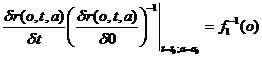
Considering (3) as valid for i = 1, . . . , m, j = 1, . . . , n the
corresponding parameters Pi
and Qj can be determined
from the As, after obtaining the
proportionality factor G, which can
be established by choosing the units for P
and Q so that, for example,
|

|
(8)
|
whereby we get
|

|
(8a)
|
The point in this banal observation
is that Pi and Qj cannot be determined
absolutely but only relative to something else, in this case P1 and Q1 respectively.
Li
can thus only be estimated through comparison with another body in L, and Ii
only through comparison with another instrument in I.
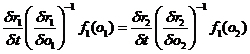
If the same instrument Ii is used for setting up the
comparison between two random bodies Lh
and Li in L, then it is
based on the two accelerations Ahj
and Aij thus expressed
according to (3):
|

|
(9)
|
The result of this comparison has
two obvious qualities:
a.
It is independent of all other
bodies in L,
particularly of the other bodies in a relevant collection L1, . . . , Lm.
b.
It is independent of which
instrument in I is used for setting up the comparison,
particularly of the other instruments in a relevant collection I1, . . . , In.
Similarly, two random instruments Ij and Ik in I are compared by
means of the two accelerations Aij
and Aik that they effect
in the same body Li, since
|
|
(10)
|
which is only dependent on the two
instruments, but neither on the other instruments in I (cf.
a.), nor on the body used (cf. b.).
7. The specific objectivity of the comparisons. All the possible
situations for observations have now been defined by means of the frame of
reference [L,I,A]: the bodies in L must be compared with regard to the accelerations (A) the
instruments in I inflict on them. And the
instruments are compared analogously.
That presupposes implicitly that the
observations take place within an isolated system so that they are not affected
by what goes on in the world outside. That is, neither by the position of the
stars, lorries driving by or high political problems. However, it is also
required that the design of the study - the necessary manipulation of bodies
and instruments, as well as the registration of the accelerations - does not
interfere in the observation situation.
This strictly isolated system is
thus completely characterised by the frame of reference [L,I,A] and the
corresponding parameters. Within this frame,
all possible As are potentially given
data - in a relevant observation situation, Aij;
i = 1, . . . , m; j = 1, . . . , n is the actual given data - while the parameters P and Q are unknown, but they are the only unknown
part of [L,I,A]. The statements a and
b then claim that, given the
relationship (3) as a fundamental foundation of the frame of reference, the parameters for two random bodies can be
compared based on what is known, i.e. observed accelerations, and the result is
unaffected by everything unknown outside the frame of reference.
That the analogous situation applies
to the comparison of instrument parameters is self-evident.
In this precise sense, we can term
the comparisons "objective". However, in both science and daily debate, this
expression is used to mean a number of things, and therefore I will tighten up
the terminology by terming the
comparisons specifically objective, that is specified by the
frame of reference.
8. Scalar latently additive differences. The analysis of Newton's
second law carried out here has its parallels in the fundamental laws of
elementary classical physics, many of which are multiplicative like (1), and in
several cases, they are followed up by analogies to the additive laws (5a) and
(6a). However, regardless of whether the latter are found or not, the specifically
objective comparison can be established through (1).
However, not only does this law
generate such comparisons. It is possible that there are objects O, other than solid bodies, that came into contact with agents A,
other than just moving mechanisms, thereby resulting in reactions R, other than just accelerations. Furthermore that, with regard to
this relationship, O, A and R are characterised entirely by unidimensional - so-called scalar -
real parameters o, a and r. Since R is considered
determined by O and A, r
has to be an unambiguous function of o
and a:
|

|
(11)
|
In the special case of the previous
example,
|

|
(12)
|
which logarithmically transformed
can be expressed additively
|

|
(12a)
|
which yields, when used on m objects, n agents and mx n
reactions,
|
 , i = 1,...,m; j = 1,...,n , i = 1,...,m; j = 1,...,n
|
(13)
|
or
|

|
(13a)
|
where the lines indicate the
logarithmic transformation.
In this additive system, which is,
of course, equivalent to the multiplicative system (12), oh and oi
can be compared by
|

|
(14)
|
which applies to every j and is therefore a specifically
objective statement. The analogous situation applies to comparison of two as.
A handy control of the additivity,
which at the same time determines the addends except for an additive constant,
can be attained by forming the average over i
and j
respectively in (13a):
|
 , ,
|
(15)
|
which yields when i is inserted (13a)
|
 , ,
|
(16)
|
For fixed j, the difference  will be constant so
that
will be constant so
that  plotted against
  gives points on a
straight line with the slope 1. Analogously for plotted against
gives points on a
straight line with the slope 1. Analogously for plotted against  .
.
However, the same reasoning also
applies if just r is dependent on o and a so that there are 3 functions
of r, o and a that satisfy the additive relationship
|

|
(18)
|
In that case, we refer to the system
[o, a, r] as a latent additive system, here presupposed
scalar, and we now know that such a system guarantees the possibility of
specifically objective comparisons between objects and between agents.
9. Condition for latent scalar additivity. Examining whether a system
of scalar variables is latent additive is, in principle, rather simple by
differentiating the equation equivalent to (18)
|
|
(18a)
|
with regard to o and a respectively to
obtain the two relationships
|
 , , 
|
(19)
|
Where f'(r) is eliminated by
division to obtain
|

|
(20)
|
which predicts that the relationship
between the two partial differential quotients of the reaction function r must form a multiplicative system.
Whether it
does form a
multiplicative system can be examined by taking the logarithms and, by
means of the technique outlined in (15) and (16), examining whether they form
an additive system. If they do, you will at the same time determine g'(o) and h'(a) - except for a multiplicative constant - and can by means of
integration form g(o) and h(a) - except for additive constants.
Since (20)
is not only a necessary but also a sufficient condition for latent scalar
additivity, the sum g(o) + h(a) must necessarily be a function of r. You can therefore finally determine f(r) from (18a).
The
sufficiency of (20) is seen in the modified formula
|
|
(20a)
|
by viewing
r(o,a) as a function  of
of  and
and  since for this
function the following equation applies
since for this
function the following equation applies
|
|
(21)
|
where the
general solutions are all (differentiable) functions of 
|
|
(22)
|
which,
when inverted to
|

|
(23)
|
is
identical to (18a).
10. Specific objectivity and latent scalar additivity. In Section 7, it
was pointed out that the generality that lies in specific objectivity within a
given frame of reference can be achieved if the reaction system is latently
additive in one-dimensional parameters. But it can be illustrated that this
condition is also necessary for specific objectivity of comparisons of objects,
provided that all three sets of parameters o,
a and r are scalar.
That a
comparison between two objects Oh
and Oi can be made
specifically objectively means first and foremost that, from their reactions Rhj and Rij on a random agent Aj, it is possible to derive a statement U{Rhj, Rij}, which is
independent of Aj but
dependent on Oh and Oi. Since objects, agents and
reactions are fully characterised by their parameters, this requires the
existence of a statement about rhj
and rij - i. e., a
function of them - that only depends on Oh
and Oi. Objectivity therefore
requires that there are two functions u
and v, each consisting of two
variables, for which
|
|
(24)
|
Using the
terminology of (11), we can write
|

|
(25)
|
so that
(24) becomes
|
|
(24a)
|
Both formulas can be used as required.
The
condition for specific objectivity set up here applies regardless of the
dimensionality of the three sets of parameters, but in the following we will -
in continuation of the previous observations - limit ourselves to reference
systems in which the parameters for objects, agents and reactions are scalar.
Furthermore,
for the analysis of what (24) implies, it will to some degree be necessary to
specialise the class of comparisons sought to be discovered. Here we limit this
class by requiring that the three functions r(x, y), u(x, y) and v(x,
y) in the studied areas for o and a have continuous partial derivatives of
the first order.
Under this
condition, it is possible to differentiate (24) with regard to each of the
three variables oh, oi and aj. According to the chain rule, this gives us
where, by
means of the two earlier equations, it becomes possible to eliminate the
differential quotients of u in the
laterr equation:
|
|
(27)
|
Since this
relationships must be valid for all oh,
oi and aj, we can in the first
instance keep aj constant,
for instance = ao. The
coefficient for, for example,  will thereby only be
dependent on oh, and we
are free to call it 1/g'(oh). Used in both components
on the left side of (27), this specialisation shows that v(oh, oi) must satisfy a partial
differential equation of the form
will thereby only be
dependent on oh, and we
are free to call it 1/g'(oh). Used in both components
on the left side of (27), this specialisation shows that v(oh, oi) must satisfy a partial
differential equation of the form
|
|
(28)
|
and using
the same reasoning as in the conclusion of Section 8, it follows that v must be a function of the difference
between
|
 and and 
|
(29)
|
that is,
of the form
|
|
(30)
|
The function v is thus latently subtractive.
In the
second instance, we let aj
vary freely in (27) but eliminate the differential quotients of v by means of (28). Thereby we get
|
|
(31)
|
But since
the left side is independent of oi
and the right side of oh,
each side must be independent of the o
in question, i.e. only dependent on aj.
We can therefore put
|
|
(32)
|
which can
be rearranged into
|
|
(33)
|
and from
this it follows that the function r
is latently additive, i.e. of the form
|
|
(34)
|
in which,
apart from (29), we have put
|

|
(35)
|
Combining this result with the
conclusion of Section 9, we have illustrated one of the main theorems of the
theory of specific objectivity:
If the parameters for objects, agents and reactions are real numbers, it
is a necessary and sufficient condition for specifically objective pairwise
comparisons of the objects that the reaction parameter is a latent additive
function of the object and agent parameter.
To this may be added that the
definition of the concept "comparison of two objects" can be extended to
include comparison between several objects and that the condition for its
specific objectivity is also the latent additivity of the reaction function.
Finally, it may be mentioned that,
due to the fact that objects and agents appear completely symmetrically, the latent additivity is also necessary and
sufficient for specifically objective comparisons between agents. The two
kinds of objectivities go together.
11. Production as determined by capital and job. Since I have not had
the opportunity to test the following on adequate data, it must not be taken
too seriously, at least not as yet. Rather, it is a sample of what it may look
like when you try to move latent scalar additivity into economics.
Production as function of capital
and job
|

|
(36)
|
is often specialised to a
Cobb-Douglas function
|
 0 < a <
1, c constant 0 < a <
1, c constant
|
(37)
|
On the surface, it does not appear
to be multiplicative, but one could say that if the exponent α was known, then
|
 , , 
|
(38)
|
would have expressed capital and job
in a new metric in which P is
multiplicative.
Using the terminology from the
previous sections, you could also say that the system (37) is latently additive
and that the transformations into additivity are
Naturally, if adequate data are
available, it is quite easy to estimate α
from them, that is, if the model fits well enough. But if possible, the
question of "in which metric P, K and A should be measured in order to bring the correlation between P, K
and A to expression into an additive
form" could also be left open.
This way of presenting the problem
would pose questions about the existence of three functions f, g
and h, for which
|

|
(40)
|
and these functions would have to be
determined empirically as indicated in Section 9.
Of course, the way of presenting the
problem may be modified, for example, as inspired by Cobb-Douglas, by entering
the ratio L = K½A and A as the variables that determine P. But to the actual idea, this is but a
detail.
I see a main difficulty in the
acquisition of adequate data for which the two - or for that matter, more -
determining variables that you have fastened on should vary freely in relation
to each other, but which often, for example when a single firm is studied over
a number of years, accompany each other. But if it is overcome, for example by
including more, differently sized firms that manufacture the same product, you
will, when latent scalar additivity is present, get objectivity into the
bargain, which should be utilisable like that of physical laws (cf. section 1),
in so far as the frame of reference can be made sufficiently comprehensive.
12. Latent additivity and probabilistic models. When, in the previous
sections, multiplicative and additive ratios, for example (3), (5) and (6),
were discussed as well as differential equations, then they are, strictly
speaking, only valid when the given data, the values of the reaction function r(o, a) are not noticeably burdened with
minors errors or other random variations.
The mathematical apparatus used for
the treatment of such variations is, as you will be aware, the calculation of
probability. You then face the task of embedding the latently additive
structures in probability models,
where the basic principle, the specific objectivity of the comparisons that are
to be made, is discovered.
Sections 13 and 14 illustrate how at
times it is possible to work towards such a model.
13. Latent additivity in percentages organised in a 4 X 4 table.
Approximately 100 years ago in his famous studies on suicide, the French
sociologist Durkheim used a peculiar technique when describing tables
demonstrating how the suicide frequency varies with two different social
factors.
The idea in his method can be
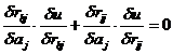
illustrated through Table 1, which is an extract of the material in Table 5.4
in Bent Bøgh Andersen (1972). Here "the time perspective" denotes the
individual pupil's attitude to planning of the future, as measured by a
questionnaire.
It is apparent that the percentages
in each row and each column are monotonously decreasing so that the traditional
"χ2 test for independence" is without interest. It can be
tempting with Durkheim to read the percentages of the table slantwise and still
find systematic progress in the figures. Details in this way of viewing the
table are described by the author of the report (p. 63), who has rescued
Durkheim's technique from near oblivion.
A more systematic analysis technique
is seemingly needed in order to arrive at a clear description of the structure
of the table. What we will do then is examine whether a latently additive
structure can be perceived behind the systematic features.
Obviously, since percentages are
locked between 0 and 100, they cannot form an additive system themselves, but
must be transformed so that, in principle, the figures achieve free mobility
between - ¥ and + ¥. This is achievable through a
so-called logistic transformation
|
|
(41)
|
where p designates a given
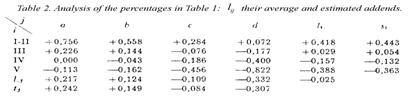
percentage. By applying it to the percentages pij of Table 1 where i
is the father's status and j the time
perspective, you get the contents, lij
= loge( pij), of Table 2.
In order to see whether this simple
transformation has succeeded in bringing forth the additivity, you can build on
the technique outlined by the forms (13a), (15) and (16) in section 8 and here
calculate the average of each row (li.)
and each column (l.j), as well as the total average (l..). If theoretically you
should have the relationship
|

|
(42)
|
- where si and lj
are constrained by setting their average to 0 - we would have to have
in which the symbol » indicates that the right side estimates the
parameter on the left side.
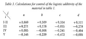
For control of whether and how well
the model fits in the present case, the estimates (43) can be inserted instead
of the parameters c, si and tj in (42). Thereby we get the "calculated values"
|

|
(44)
|
in Table 3 to compare with the
original lij in table 2,
for example by means of a diagram with the lijs
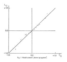
as ordinates against the corresponding  as abscises. The
result is shown in Figure 1, in which the points wind tightly around the
identity line that they were supposed to lie on if the lijs could be presented precisely by form (42).
as abscises. The
result is shown in Figure 1, in which the points wind tightly around the
identity line that they were supposed to lie on if the lijs could be presented precisely by form (42).
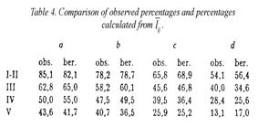
Table 4 shows how abundantly well
the percentages back-calculated from conform to the observed percentages pij.
14. Setting up an additive probability model. A precise presentation
is, of course, not possible. Percentages like pij, must at best be presumed to be subject to random
variations in accordance with the binomial law with some parameter zij. Since nij is the number of pupils
characterised by the combination (i, j) and aij denotes the number who went to the 1st
year in secondary school, the probability of this exact number must be
|
|
(45)
|
Since the expected value of aij in this distribution is
|

|
(46)
|
aij½ nij = pij½100 could be taken as an estimate of zij. Therefore lij should also be an
estimate of the logistic transformation of zij.
What the analysis in Section 13 has
shown is then that there is a good chance that
|
|
(47)
|
Solved with regard to zij, this relationship states
that
|
|
(48)
|
which with
|
 , , 
|
(49)
|
simplifies to
|
 , , 
|
(50)
|
This model is as much the same as
the one that has been widely used in recent years for analysis of individuals'
sequences of responses to a number of questions, each with two possible answers
(see, for example, chapters 12 and 13 in Ulf Christiansen and Jon Stene (1969),
henceforth referred to as GR's Textbook). However, here it is used for the
study of subpopulations.
The frame of reference from Sections
8 and 10 with objects, agents and reactions also applies here: the objects can
be the time perspectives, which are exposed to the father's status as agents
resulting in specific probabilities that pupils in the 8th school
year enter the 1st year in secondary school. To this is added the
assumption that all pupils in the (i,j)
group have the same probability zij
of ending up in the 1st year
in secondary school. In this case, this probability is determined by the
two parameters Si and Tj, i. e., through the
relationship (50), the exponential version of which (48) shows that this reaction is latently scalarly additive.
Finally, since the random factors in
the pupils' positions are presumed to be mutually irrelevant, which is
formalised as "stochastic independence", the binomial distribution (45)
follows, which, with the terminology introduced in (50), takes the form
|
|
(51)
|
This kind of application of
so-called "measurement models" is dealt with in GR's textbook under the
term "distribution analysis". The model (51) is only mentioned in passing, but
parts of its theory have been developed by Poul Chr. Pedersen (1971).
15. Separation of parameters and specifically objective estimation. The
calculations in Section 13 would have led to a specifically objective
determination of the parameters c, si and tj if (48) had been a presentation of the actual
observed relative frequencies. But since this is not the case, the question
remains whether it is possible to estimate the parameters with specific
objectivity. This will now be examined. We will restrict ourselves to the
comparison of two time perspectives j
and k based on an arbitrary status i.
Since the
groups (i,j) and (i,k) consist of different pupils, we have
the courage to assume stochastic independence between aij and aik.
According to (51), we then have
|

|
(52)
|
In this
expression, Si appears to
the power aij + aik, and the probability for
a specific value r of this sum is
found by writing down the probability p{aij, aik} for every single
possible value pair (aij, aik) with this sum and adding
them together. Thereby, we get
|

|
(53)
|
in which
the polynomial
|
|
(54)
|
is
homogeneously of degree r in Tj and Tk.
If the
probability (53) is divided by p{aij, aik} given in (52), you
get the conditional probability for exactly those two quantities aij and aik, given that their sum is r:
|
|
(55)
|
Here it
can be seen that this procedure eliminates Si
so that the probability (55) does not depend on other parameters than the ratio
between Tj and Tk.
This ratio
can thus be estimated based on any i,
and all of these estimates (in this case 4) must be statistically compatible.
Whether
they are statistically compatible can in specific cases be tested by comparing
the individual pairs (aij,
aik) with the total (aoj, aok). However, the formulas required for this, as well as the extended system of
formulas that simultaneously involves all (16) pairs (i, j), will not be
treated here.
At this point, the main result must
be mentioned. The first part is a generalisation of (55):
Any set of Ts can be estimated and evaluated independently of both the
other Ts and all Ss and vice versa, in so far as the model (51) together with
stochastic independence of the observed counts is correct.
The model hypothesis can be tested independently of all the parameters.
For the stochastic model mentioned here, the same applies as was emphasised
for the deterministic models in
Section 7. The only unknown factor in the
reference system is the parameters and comparisons between objects as well as
agents (cf. form (55)) can be made based on what is known - i.e. the
observed data (aij, given nij) - unaffected by everything that is not known within the reference system.
The statistical statements about the parameters that are based on this can
therefore be termed "specifically objective".
An obvious question is then which
models have this remarkable quality. Mathematically, the possibilities are
extremely limited. Keeping to the present situation with only two possible results in each instance
and stochastic independence between the outcomes of the instances, the probability model given
in (45) and (50) is - except
for trivial transformations - the only
model that allows specifically objective separation of the object and agent
parameters.
We refer to chapter 13 in G.R.'s
Textbook for the proof.
16. Orientation towards processes. The theory for specific objectivity
and latent scalar additivity developed in Sections 1-7 and 8-10 as well as the
two applications in Sections 11 and 13-15 only treat stationary systems where
all reactions are determined by two fixed sets of parameters.
Through the next two examples, we
will approach the problems connected to changes in a system. The stochastic
problems are, however, far deeper in such areas than in the sociological
example. Therefore, I must limit myself to suggestions on this occasion.
In the treatment of two data sets,
we will disregard these problems and restrict ourselves to "the broad outlines"
- whereby they will become examples of what I have called "numerical
statistics" in a different context. Hereby, structures appear that must be
implemented in future studies into the "stochastic processes" that may have
generated the data.
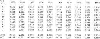
17. Preliminary analysis of a number of wage development curves. From
the publication Statistikken by Arbejdsgiverforeningen
(the Employers Association) from the years 1953-69, P. Toft-Nielsen and Steffen
Møller have extracted the hourly wages per year in 9 large areas or
"industries" and made the material available to me. Sorted according to the hourly
wages in 1969, it is reproduced in Table 5, and illustrated in Figure
2 for four characteristic cases. The remaining cases proceed according to the
pattern in the three curves, while the direction of the fourth curve (F) cuts
across all the other 8. These eight curves are at different levels and with
different slopes, but even though some of them can be practically identical,
they do not cut each other. The
singular F cuts across several of the 8 curves, but it has the typical
progression - in the beginning a weak increase, which is gradually replaced by
a stronger and stronger increase that brings about a strongly curved sequence
with the concavity facing upwards - in common with the other 8, only the slope
is weaker.
Here it seems there is cause to look
for a common structure for all nine industries, possibly a latent scalar
additivity. This possibility is tested - however, in reality only for the sake
of completeness - using the method indicated in Section 9. The result (not
demonstrated here) was completely negative.
|
Table 5. Average hourly wages xi(t)
for 9 industries for the years
|
|
|
|
This was, though, exactly what was
to be expected since the wages in the successive years are not a fixed system
where each year's hourly wages is determined regardless of the level in the
previous years. It is a system in motion: through collective bargaining and
wage drift, each year's hourly wages in an industry emerge from the hourly
wages of the previous years.
As a first and possibly applicable
approximation, we will examine whether the wage increase between two times t1 and t2 for the individual industry (no. i) can be formalised as a continuous process, the direction of
which at a given time t is determined
by three factors: the hourly wages of the industry at time t, the current financial conditions common to all the industries,
and the special conditions that apply to the industry in question which are
considered constant over the term of years.
Designating the hourly wages of the
industry at the time t, x1(t), the speed of the increase x1'(t) will depend on x1(t) itself,
on a "general economical development function" f'(t) for all the
industries, and on a constant parameter bi,
which is particular to the industry in question.
If there is latent scalar additivity
or, in this case more conveniently, latent scalar multiplicativity in this
system, there must be two such functions: first, f of the reaction x1'(t), and second, h of the agent x1(t) so that
|
|
(56)
|
Determining the unknowns - the
functions f, g and h and the constants
bi and g'(t)
- directly from x1'(t) and x1(t) as exactly given would perhaps be
theoretically possible, but since we would then go up to differential quotients
of both 3rd and 4th order, it will be unworkable when the
data in question are burdened with what must be considered measurement errors
and other random fluctuations.
At present, we will instead attempt
the very simple assumption
|
 , , 
|
(57)
|
that is, use as our starting point
the equation
|
|
(58)
|
which is integrated into
|
|
(59)
|
in which ai is an integration constant.
Testing this model simultaneously
with an empirical determination of the function g(t) and the two sets of
constants ai and bi is a relatively simple
matter: if the average of
|

|
(60)
|
is calculated over the industries,
we get
|
|
(61)
|
If a g(t) exists, we can as
such simply take y.(t) (or a linear transformation of it)
which, when inserted into (59), gives
This equation states that if the
model (59) holds and we draw a diagram for each industry with the successive
values of yi(t) for t = 1953, . . . , 1969 as ordinates against the corresponding
values of y.(t) as abscissas, then the points must lie on a straight line with
the slope of bi'. We can
choose as origin, for example, the ordinate on the line with the abscissa  = the average of y.(t)
over t. We therefore set
= the average of y.(t)
over t. We therefore set
|

|
(63)
|
In practice, we will, of course,
only get a sort of estimate of ais,
bis and g(t),
and the control can at best only provide points that lie more or less closely
around straight lines.
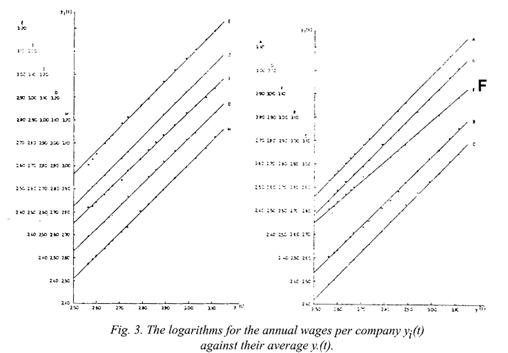
Table 6 shows the logarithms for the hourly wages as well as their
average over i, and Figure 3 shows
the control diagrams with parallel staggered ordinate zeros for the different
industries.
|
Table 6. The logarithms for the
hourly wages yi(t) = loge xi(t) in Table 5.
Average y.(t) of yi(t)
over i as well as slope bi and intercept ai of the
lines in Fig. 3.
|
|
|
|
We can see that the points cling
fairly closely round the respective straight lines so that the model (59), and
thereby also (58), must be said to offer a satisfactory representation of the
present data.
It is noted that, as expected, the
slope for the industry F is a great
deal smaller than for the other eight, but also that differences of some
importance between these slopes can be seen.
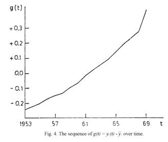
The estimate of the function g(t)
is given as the bottom line in Table 6, in which the estimates of positions ai and slopes bi are found as the two columns furthest to the right.
For the sake of completeness, the
discovered function is drawn up in Figure 4, from which it can be read that in
the first five years, the sequence of g(t) corresponds to an annual increase in
wages of approximately 5% while in the last 5 years, it was approximately 11%,
for F somewhat lower and for A a little higher.
18. Objective evaluation of the process parameters. With the discovered
results, it is completely clear, including technically, why the first test
broke completely down: xi(t) as determined by time and industry
contains a scalar parameter g(t) per
time, but a two-dimensional parameter (ai, bi) per industry, while the theory in sections 1-10 presupposes that
there are only one-dimensional parameters.
However, viewing the wage
development as a process brings out the multiplicativity, as illustrated by
(58) re-expressed as
|
|
(64)
|
when viewing loge xi(t), and not xi(t) itself, as the thing that changes.
Employing this "process" point of
view, we have reached the latent scalar additivity of two sets of parameters,
the industry parameter bi
and the general sequence parameter g'(t), which can then be evaluated
specifically objectively. Conversely, the determination of ai falls outside the developed theory of objectivity.
Incidentally, the statement (64)
corresponds to the fact that in wage negotiations and wage drift, people may talk about actual money, however in
reality, they think in terms of
relative wage increases (cf. the concluding remark in Section 17).
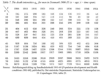
19. Structure in mortality data. The third example drawn from
demographics is about the variation of the death intensity with age for men in
Denmark in the years 1906-1955, the age x (5-75 years old) for every 5th
year and the calendar year t grouped
in intervals of 5 years. The death intensity is, in principle, to be understood
here as the number calculated per 100,000 among those who in the time span (t, t+5) turned x years old who died before their next birthday.
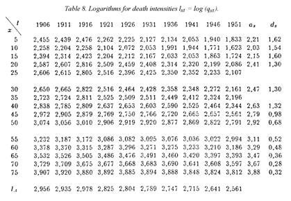
The basic data in Table 7 naturally
shows very large variation with age, which complicates immediate comparisons
between the age levels. As an attempt to compensate for it, we take the
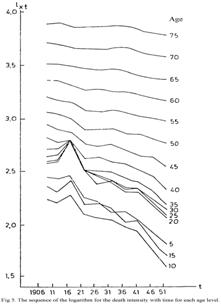
logarithms shown in Table 8; the effect is illustrated in Figure 5, which shows
for each age level how loge qxt
has changed over the course of 50 years. The sequences are fairly steady,
however, for the ages up to 40 interrupted by strong peaks upwards for t = 1916, i.e. for the five-year period
1916-1920 with the two great epidemics of "the Spanish flu". But outside this
period - and apparently without major lasting effects of it - we see a steady
decline over the years, strongest for children and youths, still considerable
from ages 40 to approximately 60, but flattening more and more for the elderly.
This observation tempts us to seek a
structure, but taught by the experience with the hourly wages, we will not
directly seek a latently additive structure. However, regardless of the lack of
a basis such as (58), we must ask purely geometrically whether the curves in
Figure 5 - similarly to the logarithmical wages of the 9 industries - can be
linearly transformed onto each other.
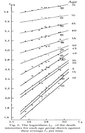
The bottom row in Table 7 gives us
the average ("unweighted") over ages for each time-interval, and with these as
abscissas drawn in Figure 6 for each age level, it becomes a diagram with the
values of lxt = loge qxt as ordinates. (x = 25 and x = 35 are omitted as
they almost coincide with x = 20 and x = 35 respectively.) The points for
1916 are framed by circles and are in general level with the other points,
which otherwise for each age level gather around a straight line. The
variations are obvious enough, and it is really not unthinkable that another
structure layer could be revealed through careful examination. But the main
thing is that, in any case, there is an obvious primary structure that can be
expressed as the linear relation of lxt
to l.t for each age
group:
|
 , , 
|
(65)
|
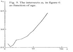
The slope of the straight lines dx and the positions ax determined as ordinates
for the abscissa for  = the average over t of l.t
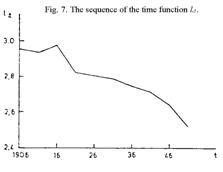
is read and inserted as the two last columns in Table 7. The sequence of the
time function l.t is shown
in Figure 7; except for a peak upwards in the t = 1916 curve mentioned above, it shows a steady decline. Figure 8
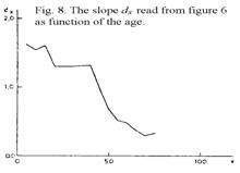
shows that in broad outline, the slope dx
decreases monotonously with age, however with a plateau from ages 20 to 40; the
fluctuations may be real, but they may partly be due to the uncertainties in
the graphical determination of the slopes, since it is sensitive to the
variations of the points around the lines, which are not quite small. This
variation does not much affect the reading of the positions ax which also, as illustrated
in Figure 9, shows a steady monotonous sequence except the fall from ages 5 to
10 which, however, is quite real and already emerges clearly from Figure 5.
= the average over t of l.t
is read and inserted as the two last columns in Table 7. The sequence of the
time function l.t is shown
in Figure 7; except for a peak upwards in the t = 1916 curve mentioned above, it shows a steady decline. Figure 8
shows that in broad outline, the slope dx
decreases monotonously with age, however with a plateau from ages 20 to 40; the
fluctuations may be real, but they may partly be due to the uncertainties in
the graphical determination of the slopes, since it is sensitive to the
variations of the points around the lines, which are not quite small. This
variation does not much affect the reading of the positions ax which also, as illustrated
in Figure 9, shows a steady monotonous sequence except the fall from ages 5 to
10 which, however, is quite real and already emerges clearly from Figure 5.
20. A comment on the discovered structure. The structure relation (65)
is of quite a singular form as it states that in the period in question, the
death risk for men was by and large only determined by their age x and the time t when they were that age, while what had happened before their
lifetime - within hygiene, medicine, technology, social conditions etc. - in
any case only played a secondary role with regard to the current condition in
society at the time in question.
Is it possible that such a peculiar
result could be a, however almost incredible, statistical trick that these data
from Denmark in just those 50 years have played on us?
However, to this can be added that
approximately 10 years ago, P. C. Matthiesen carried out a similar study of
Swedish data and found a quite similar result (unpublished). Furthermore that
among the mortality data from a number of countries found in the publication
United Nations (1955), 19 countries that had at least 4 registration times were
chosen for a preliminary study in a seminar at the Statistisk Institut (Statistical Institute) in the Spring of
1969 and later analysed more in depth by Peter Allerup in an exam paper:
everywhere, the same structure was found.
It therefore seems that we will have
to resign ourselves to the structure revealed in the Danish data - if nothing
else then at least as a first step towards the formulation of a structure describing the effect of age on mortality
under different local and temporary conditions that is common for many places
in the world.
21. The problem of objectivity in the case in question. With regard to
the problem of objectivity, it must first be noted that, when viewed locally,
we have in (65) a situation similar to the one in (64), i.e. a one-dimensional
parameter lt per time, but
a two-dimensional parameter (ax,
dx) per age level. It is
not covered by the previously developed theory, but it invites an extension of
the frame of reference so that the restrictions of one-dimensionality of the
parameters for objects, agents and reactions are loosened. An extension to
higher dimensions does exist, but only under the condition that all 3 kinds of
parameters have the same dimension.
This is a restriction there may be cause to attempt removing.
However, just as in the wage
example, we can apply the point of view that what is observed, in this case the
death risk for men at a given age, is something that changes over time, and for
this change in the time span (t1,
t2), we have according to
(65)
|

|
(66)
|
that is, latent additivity and
thereby specific objectivity.
Now the death intensities - or, if
you will, their mathematical correlate - are defined as the logarithmical
differential quotients of the share of the population - at a given time - who
have survived given ages. Designating this share Lxt, we get
|

|
(67)
|
|
|
But hereby, we have already
introduced a process point of view: how the population dies out with age.
What is added in (66) - or its differential counterpart
|
(66a)
|
is also the application of the
"process" point of view to the time sequence.
We then reach the conclusion that if
the purely static point of view, i.e. the distribution of the population on age
at a given time, is replaced with the process point of view for changes of the
death risk with both age and time, then in the observed case, we achieve
specifically objective separation of the remaining scalar parameters.
22. Specific objectivity in processes? The analyses of the wage
development within the industrial sector in the years 1953-69 and of the
changes in the death risk for men in Denmark in the years 1906-55 pointed at
the possibility for achieving specific objectivity in cases where there have
been changes during the observation period and where each observation is
therefore based on that or the previous periods.
They pointed in particular to the
importance, as a condition for achieving latent additivity, of not taking the
actual wages or actual risk of mortality respectively for the reaction, but
rather the changes in them.
These two cases must be said to be
kinetic when reference is only to changes over time, not to the influences that
brought them about. But kinetic and dynamic phenomena can be summarised under
the term processes where agents can
be actual influences as well as time and time intervals.
23. The dynamic problem. In order to gain insight into the dynamic
problem, we return to the solid bodies that are affected by mechanical moving
instruments. However, we shall take the discussion a little further.
At a given time, a body L moves in relation to Earth with a
velocity V0 that is
changed to V1 under an
influence in the direction of movement by an instrument I which gives it an acceleration of A = V0 - V1.
In the previous discussion (Sections
2 and 3), we found that this acceleration is proportional to a parameter for
the instrument, its "force", and vice versa proportional to a parameter for the
body, its "mass".
The body, which was first in a
condition where it had the velocity V0,
is brought by the influence to a new condition where it has the velocity
|

|
(68)
|
where F1 designates the force of the instrument and M the mass of the body, cf. section 3,
forms (3) and (4).
But the body in its new condition
can now be influenced by another (or the same) instrument with the force F2, receive the acceleration GF2½M and
thereby be brought to a new condition with the velocity
|
|
(69)
|
cf. equation (5a). And so forth.
Through n such influences, the
initial velocity V0 is
gradually changed into
|

|
(70)
|
Throughout these changes, the body
retains its permanent parameter, the
mass M, while the condition parameter, the velocity V, goes through changing values.
24. The frame of reference for processes. We can now set up a frame of
reference for processes in continuation of the one set up for statics in
section 6.
Once again, we have objects O, agents A and reactions R, but to
this is added that an object can exist in different conditions T and that the transition from one
condition to another happens through a transformation that is brought about by
the reaction R effected by an agent A on the object in the previous
condition. The sequence can be thus schematically presented:
|

|
(71)
|
in which the upper index of O is the identification of the object,
which is constant during the whole process, while the lower index of O marks the changing conditions.
The purpose of the following
analysis is to develop tools for comparison within this frame of reference:
comparisons between objects with reference to how the observed kinds of
processes elapse. In this, it is implied that the problem is not the
description of a single sequence, for example a single TIME SERIES, say in the
price development for potatoes in Denmark from 1919 to 1955, but rather the price
development for many kinds of vegetables and other foods, possibly other goods.
Furthermore, the comparisons are between conditions, regardless of the objects
where they occur. And finally, the comparisons are between agents as they work
on any conditions with any objects.
25. Parameterisation and specific objectivity for processes.
Parameterisation encompasses agent parameters a, the permanent parameters of the objects o and their condition parameters t, as well as the parameters of the reaction r, which in any given situation are unambiguously determined by the
3 other parameters:
|

|
(72)
|
Similarly to what was done in the
static example in section 10, we designate here a comparison of, for example,
two objects with the parameters o1
and o2 specifically
objective if it is independent of the other parameters in the frame of
reference. Since the statement must be based on what is known, i.e., the
observed reactions r, the demand
implies the existence of a function u
of the two rs, which is dependent on
the two o's that are to be compared.
Therefore
|

|
(73)
|
cf. formula (24).
Still limiting ourselves to scalar
parameters, it can be demonstrated that if
specific objectivity is demanded in all 3 directions, the reaction r must be
latently additive in all 3 variables.
The proof of it runs almost parallel
to the one that was given in section 10.
By
alternately differentiating (73) with regard to all 4 variables, we get 4
equations of which the two differential quotients of u with regard to r1
= r(o1, t, a) and r2 = r(o2, t, a) can be eliminated. Hereby we get
|
|
(74)
|
and the
analogous equation by differentiation with regard to a. If we give t and a special values t0 and a0
and introduce the designation
|
|
(75)
|
we get
|
|
(76)
|
and the
analogous equation. From this it follows that these four expressions are only
dependent on t and a, and we can therefore gather the
equations in
|
|
(77)
|
In the
same way, we get for the specific objectivity in the two other directions
|
|
(78)
|
and
|
|
(79)
|
But if the
three sets of equations are to apply simultaneously, they must be reducible to
one set of the form
|
|
(80)
|
which with
as new
variables and with the designation
|

|
(82)
|
is reduced
to
|
|
(83)
|
with a
random function of  as the complete solution.
26. Status and perspectives. My purpose in this retirement lecture was
to give the audience insight into the trains of thought that studies within
psychology in the '50s and taking over the Chair in Theoretical Statistics
as a Tool within Social Sciences provoked me to take up on a wide basis.
As far as it has been worked out,
the theory is already quite comprehensive, so on this occasion, heavy cutting
was necessary. This has been carried out in two directions, partly through a
limitation to cases where all the parameters are one-dimensional, which leads
to both results and proofs becoming relatively simple; and partly by
restricting ourselves to the situation where only 2 different responses are
possible in indeterminate cases.
The one-dimensionality restriction
ensures that the reactions - which in the indeterminate case are the
probability distributions of the two possible responses - become latently
additive. And just two possible responses carry forward into as simple a
distributional form (50) as possible.
If the dimensionality model is
extended but it is maintained that the three kinds of parameters - for objects,
agents and reaction - must have the same dimensionality, then the deduction of the
differential equation (28) still applies when the terms used are interpreted as
vectors and matrices. But from this, a multi-dimensional latent additivity only
follows under much more restrictive conditions, which, by the way, cannot be
said to have been completely mapped yet. However, one highly applicable
sufficient condition is available.
If in the stochastic problem the
range of possible responses is extended beyond 2, the above mentioned sufficient
condition leads to a mathematically extremely limited, yet in practice still
highly comprehensive, class of distributions, the so-called "measurement
models". Furthermore, these models, which naturally encompass the simple
dichotomous model (50) as a special case, can be extended to cases where the
responses can be distributed over the entire real axis in the plane or in
space, and thereby they give us a considerable extension of the classical
statistical arsenal.
An extension in a third direction,
which has indeed been predicted but which has as yet not been intensively
cultivated, is beginning to make itself felt. It involves interactions between
more kinds of elements than objects and agents. H. Scheiblechner (1971)
recently called attention to the extension as an important tool within
sociology and social psychology, and it will certainly be completely essential
in analyses of financial systems.
The kind of mathematical problems
that this extension causes has already crept into the treatment of the process
problem in section 25 where there is a correlation between 3 kinds of
parameters: one for agents and two for objects, i.e., a permanent one for the
objects as such and one for their changing conditions.
This modest glimpse into the theory
of processes opens up wide perspectives since all the available results from
the objectivity of statics can be transferred directly onto the processes -
also those where the relationship takes place between more than two kinds of
elements. It will apply to both deterministic processes and stochastic
processes so that the measurement models are carried into "measurement
processes".
With all of this available to us, we
will have an instrumentarium with which many kinds of problems in the social
sciences can be formulated and handled with the same types of mathematical
tools that physics has at its disposal - without it becoming a case of
superficial analogies.
But why stop at social sciences. My
vision stretches to all sciences where
the subjects are comparisons that must be objective.
References
Andersen,
Bent Bøgh (1972) Aspekter af
den"kulturelle" barriere mod uddannelsessøgende. [Aspects of the "cultural"
barrier to students.] Socialforskningsinstituttet, Studie 21. Copenhagen.
Christiansen, Ulf & Jon Stene
(1968/69). G. Rasch's lærebog i
teoretisk statistik. (GR's Textbook on theoretical statistics) Two volumes,
Copenhagen.
Jammer, Max (1957) Concepts of force. Cambridge, Mass.
Jammer, Max (1961) Concepts of mass. Cambridge, Mass.
Pedersen,
P.C. (1971) Analyse af gymnasiefrekvens for befolkningsgrupper opdelt efter
indkomst og social status. Tillæg II til Erik Jørgen Hansen: Ungdom og Uddannelse. [Analysis of the secondary spectrum of the population
classified by income and social status. Supplement II to Erik Jorgen Hansen: Youth
and Education.] Socialforsknings-instituttet, Publikation 47,
Copenhagen.
Rao, C.R. (1958) Some statistical
methods for comparing growth curves. Biometrics
14, 1-17.
Scheiblechner, H. (1971) The
separation of individual- and system-influences on behaviour in social
contexts. Acta Psychologia 35,
442-460
United Nations.(1955) Age-Sex patterns of Mortality.
Population Studies. No. 22. New York
[Bolding and formatting added by Editor]
 ,
, ,
,