Comparing Measures: Scatterplots

Comparison of measures is frequently required. Item calibrations are compared when tests are equated to investigate stability. Person measures are compared to investigate change. Here are some techniques of comparison.

A necessary step before final conclusions can be drawn is to establish and maintain the frame of reference. Suppose the pre-test is Form E and the post-test is Form H. Simply subtracting a mean ability measure at pre-test from a mean ability at post-test is misleading as a measure of change for many reasons. The most obvious is that pre-test measures are relative to Form E and post-test measures are relative to Form H. The two Forms must be equated into a single frame of reference, i.e., with a shared origin and scale. Only then can valid comparisons between pre- and post-test measures be made. This equating may be an iterative procedure in which the following techniques can help.

A. Numerical comparisons. A.1 Direct comparisons:
If Bn is the measure of subject n, and Bm the measure of subject m, the obvious comparison is Bn-Bm. If SEn and SEm are the standard errors of Bn and Bm, then the SE of Bn-Bm = sqrt((SEn^2+SEm^2). A two-tailed test of the null hypothesis "Bn-Bm=0" is rejected at the .05 level when
|Bn-Bm| >= 1.96*sqrt((SEn^2+SEm^2)
>= 2.8 * SEn when SEn = SEm,
and at the .01 level when
|Bn-Bm| >= 2.58*sqrt((SEn^2+SEm^2)
>= 3.7 * SEn when SEn = SEm.

A.2 Normative comparisons:
It is often of interest to discover whether, as a group changes, individuals are changing faster or slower than their group. Suppose B1 is the measure of a subject at time 1, when the mean of the N measures is G1, and B2 is the measure of the same subject at time 2, when the group mean is G2. Then the gain of the subject relative to the group is (B2-G2)-(B1-G1). The error variances of the () terms have the form
SEBG1^2 = SEB1^2 + SDG1^2/(N-1).
The SE of the gain = sqrt((SEBG1^2+SEBG2^2).

A.3 Comparisons requiring rescaling:
Tests X and Y contain some equivalent items, but, due to different candidate behavior, rating scale specifications or analytical decisions, the logit units of the measurement scales estimated for the two tests have different lengths.

Suppose there are C items common to both tests. Their mean and variance in Test X are MX and VX, and in Test Y, MY and VY. Then the rescaling factor to place measures on Test Y into the scale of Test X is
SCALEYX = sqrt((VX/VY)
so that
B'Y = (BY - MY)*SCALEYX + MX
with
SE'Y = SEY*SCALEYX
Comparisons can now be made between BX and B'Y in the metric of Test X.

A.4 Evaluation of group stability:
Suppose there are C common elements in tests X and Y. Whether to attribute the inevitable differences in pairs of measures solely to measurement error is a statistical question. A test of the null hypothesis that the differences are attributable to measurement error is the homogeneity chi-square:

B. Graphical comparisons.
B.1 Graphing without common scaling:
The numerical calculations can be summarized in a scatterplot of measures and confidence bands. Each element has two measures, BX and BY, and two standard errors, SEX and SEY.

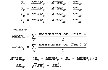
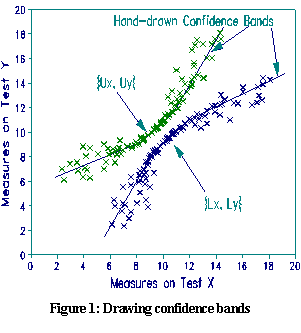
Plotting confidence intervals is a two-stage process. For conventional 95% two-tailed confidence bands, the pairs of points are located at {UX, UY} for the upper confidence band and {LX, LY} for the lower band, where

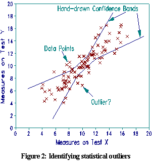
When you plot the {UX, UY} points, they will form a curved cloud (Figure 1). The points are exact, but provide too much detail. To expedite conceptualization, draw a smooth curve through these points with a thick felt-tip pen or computer drawing tool. Then erase the points. Repeat this for the {LX,LY} points. This draws the 95% confidence bands. Now plot your {BX,BY} data points (see Figure 2 (in printed text)). The identity line goes through {MEANX+AVGEX, MEANY+AVGEY}.

B.2 Graphing with local scaling:
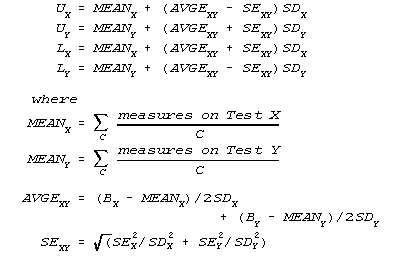
In Figure 2, the best fit line goes through points {MEANX+AVGEX-SDX, MEANY+AVGEY-SDY} and {MEANX+AVGEX+SDX, MEANY+AVGEY+SDY}. If this forms a noticeable angle with an identity line, then plot the confidence bands with the X and Y axes separately scaled. The locally scaled confidence bands are plotted in the same way as in B.1, but using these values:

The best fit line now falls evenly between the bands.

Comparing measures: scatterplots. Luppescu S. … Rasch Measurement Transactions, 1995, 9:1 p.410

Rasch Books and Publications
Invariant Measurement: Using Rasch Models in the Social, Behavioral, and Health Sciences, 2nd Edn. George Engelhard, Jr. & Jue Wang	Applying the Rasch Model (Winsteps, Facets) 4th Ed., Bond, Yan, Heene	Advances in Rasch Analyses in the Human Sciences (Winsteps, Facets) 1st Ed., Boone, Staver	Advances in Applications of Rasch Measurement in Science Education, X. Liu & W. J. Boone	Rasch Analysis in the Human Sciences (Winsteps) Boone, Staver, Yale
Introduction to Many-Facet Rasch Measurement (Facets), Thomas Eckes	Statistical Analyses for Language Testers (Facets), Rita Green	Invariant Measurement with Raters and Rating Scales: Rasch Models for Rater-Mediated Assessments (Facets), George Engelhard, Jr. & Stefanie Wind	Aplicação do Modelo de Rasch (Português), de Bond, Trevor G., Fox, Christine M	Appliquer le modèle de Rasch: Défis et pistes de solution (Winsteps) E. Dionne, S. Béland
Exploring Rating Scale Functioning for Survey Research (R, Facets), Stefanie Wind	Rasch Measurement: Applications, Khine	Winsteps Tutorials - free Facets Tutorials - free	Many-Facet Rasch Measurement (Facets) - free, J.M. Linacre	Fairness, Justice and Language Assessment (Winsteps, Facets), McNamara, Knoch, Fan
Other Rasch-Related Resources: Rasch Measurement YouTube Channel
Rasch Measurement Transactions & Rasch Measurement research papers - free	An Introduction to the Rasch Model with Examples in R (eRm, etc.), Debelak, Strobl, Zeigenfuse	Rasch Measurement Theory Analysis in R, Wind, Hua	Applying the Rasch Model in Social Sciences Using R, Lamprianou	El modelo métrico de Rasch: Fundamentación, implementación e interpretación de la medida en ciencias sociales (Spanish Edition), Manuel González-Montesinos M.
Rasch Models: Foundations, Recent Developments, and Applications, Fischer & Molenaar	Probabilistic Models for Some Intelligence and Attainment Tests, Georg Rasch	Rasch Models for Measurement, David Andrich	Constructing Measures, Mark Wilson	Best Test Design - free, Wright & Stone Rating Scale Analysis - free, Wright & Masters
Virtual Standard Setting: Setting Cut Scores, Charalambos Kollias	Diseño de Mejores Pruebas - free, Spanish Best Test Design	A Course in Rasch Measurement Theory, Andrich, Marais	Rasch Models in Health, Christensen, Kreiner, Mesba	Multivariate and Mixture Distribution Rasch Models, von Davier, Carstensen

Forum

Rasch Measurement Forum to discuss any Rasch-related topic

Go to Top of Page
Go to index of all Rasch Measurement Transactions
AERA members: Join the Rasch Measurement SIG and receive the printed version of RMT
Some back issues of RMT are available as bound volumes
Subscribe to Journal of Applied Measurement

Go to Institute for Objective Measurement Home Page. The Rasch Measurement SIG (AERA) thanks the Institute for Objective Measurement for inviting the publication of Rasch Measurement Transactions on the Institute's website, www.rasch.org.

The URL of this page is www.rasch.org/rmt/rmt91c.htm

Website: www.rasch.org/rmt/contents.htm