Investigating Drift Displacement in Rasch Item Calibrations

Item drift analyses that use displacement have reported displacement distributions symmetrically distributed around zero (Jones and Smith, 2006). Approximately equal numbers of items appear to drift in both a positive (harder) and a negative (easier) direction, despite hypotheses suggesting systematic drift in one direction. A portion of this displacement distribution can be shown to be statistical artifact resulting from the way the statistic is calculated.

Displacement is a useful statistic generated from the Winsteps analysis program. The displacement statistic "approximates the displacement of the estimate away from the statistically better value which would result from the best fit of your data to the model." (Linacre, Winsteps User Manual). In any analysis featuring anchored items, Winsteps simultaneously performs a free (unanchored) parameter estimation for all of the items. The displacement statistic results from a direct comparison of the anchored difficulty value with the value from the free estimation arising from the current data. Due to the re-centering procedures in Winsteps, the free parameter estimates are constrained to be centered around a mean of 0. Accordingly, all displacement values also sum to 0. As a result, in a dataset featuring systematic drift in one direction (i.e. easier), it is possible to observe, in stable items, drift in the opposite direction (i.e. harder) resulting from a statistical artifact.

Since the displacement statistic contains an artifact that does not represent actual item difficulty drift, the interpretation of the statistic becomes problematic and its usefulness is diminished. Simulation data was used to replicate certain conditions of item difficulty drift and to assess the impact of these drift conditions on the displacement statistic and its interpretation.

The candidate sample was chosen to have a standard normal distribution N(0,1). Three candidate samples were selected, one having 200 individuals, one having 500 individuals and one having 1,000 individuals. Three item samples were also selected, each having a standard normal item difficulty distribution N(0,1). The item sample sizes were 30 items, 100 items and 200 items. Each candidate sample size was then matched against each item sample size, resulting in nine combinations. The Promissor simulator (Becker, 2006) was used to generate an initial response string data sample for each of these combinations using Rasch probability as the basis for assigning a right/wrong response for each candidate/item interaction. The nine response strings generated by the above procedure were analyzed using the Winsteps program, and item difficulty calibrations were obtained for each item as it was used in each of the nine combinations. These item calibrations were then used to create item anchor files to be used in subsequent drift analyses.

In order to minimize the impact of outside variation, the same response string data sample was used to simulate item drift. Answers were systematically changed in the response strings to simulate a drift in an easier and/or harder direction by changing answers from wrong to right or vice versa.

The number of items that were simulated to drift was systematically varied. In the first condition, 10% of the items were simulated to drift. In the second condition 20% of the items were simulated to drift. In the final, most extreme condition, 50% of the items were simulated to drift. The first two conditions are probably more reflective of normal drift conditions. The final condition would be more reflective of a serious security breach.

Within each of the above conditions the direction of drift was also varied. In one situation, the drift was all in a single direction with the items becoming easier. In the second situation, the drift was symmetrically balanced with half the items drifting easier and half the items drifting harder. In the final situation, the drift was asymmetrical with 70% of the items drifting easier and 30% of the items drifting harder. The final condition is a combination of the first two with more emphasis on the condition of compromised items.

Combining the 9 candidate/item combination with the 3 percentages of drift and the 3 directions of drift resulted in 81 unique conditions that were simulated.

To simulate drift, the desired number of items and candidates was randomly selected without replacement from the total candidate and item samples. Each response string was examined and, for each interaction of a selected candidate and a selected item, the answer was examined and changed appropriately to simulate the desired drift. If the answer for that particular candidate/item interaction was already in the direction of the desired drift no action was taken.

The modified data sets were then reanalyzed using Winsteps. The item difficulties of all of the items were anchored to the item calibrations obtained from the initial analysis. The impact of the drift on the displacement distribution was then assessed.

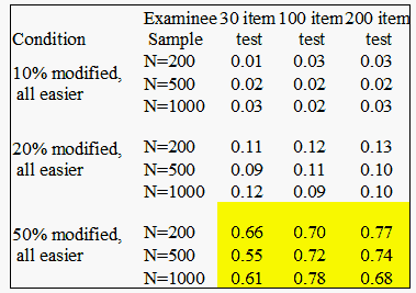
Table 1. Mean displacement values for hypothetically stable items (unidirectional drift)

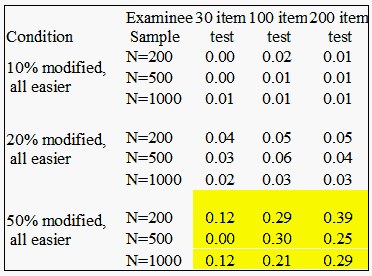
Table 2. Mean displacement values for hypothetically stable items (asymmetrical drift)

The results of the simulations and analyses are summarized in Tables 1 and 2. Tables 1 and 2 contain average displacement values observed on items whose response strings were not modified to mimic drift (i.e. items hypothesized to remain stable over time). The mean displacement values are replicated for each condition of the simulations. Table 1 represents simulation cases where hypothetically drifting items were all displacing exclusively in a negative (easier) direction.

Table 1 also demonstrates that when systematic drift in one direction was present in a data set, then hypothetically stable items in every test condition exhibited artificial positive displacement. The artifact was more pronounced in conditions with increased test length and increased proportion of drifting items. The amount of artificial positive drift appeared to be unrelated to examinee sample size. To provide some indication of significance, we compared the Table 1 displacements to the value corresponding to two times the average standard error (SE) of item calibrations for each examinee sample condition (for N=200, 2*SE = 0.34; N=500, 0.22; N=1000, 0.14). Highlighted cells in Table 1 reflect displacement values that might be interpreted as significant because they are more then more than two SE from the original calibration. Obviously, these potential false positives occur exclusively in the extreme simulation conditions where 50% of the test items were modified to show easier drift.

Table 2 summarizes simulation cases where hypothetically drifting items were displacing asymmetrically (70% easier, 30% harder). The patterns of average displacement for hypothetically stable items (i.e. items whose response strings underwent no modification) are similar in Table 2, yet not as pronounced. The artificial positive displacement is detected more in data sets with a large amount of systematic drift. Again, artifact that could be interpreted as significant is highlighted. The problem posed by artifact is somewhat ameliorated in the simulations where all of the drift was not in one direction.

Not surprisingly, in simulations featuring balanced drift - or equal amounts of drift in both directions - the problem of artifact was completely ameliorated. In these simulations, the average displacement value for items hypothesized to remain stable was consistently 0, so their values are not tabulated. This statistical artifact is a result of the way the displacement statistic is calculated and the fact that the results are mean centered. In situations in which the degree of drift is symmetrically distributed in both an easier and a harder direction, the impact is relatively minor. As the drift becomes more asymmetrically distributed, the impact of the artifact becomes more noticeable so that non-drifted items may be flagged as significantly and substantially drifted.

However, the impact can be easily detected by plotting the displacement against the sequence number. Items with a very consistent drift are items that are being affected by the artifact. It is recommended that such a plot be used as a part of any drift analysis. It may also be possible to detect the artifact during the displacement calculation by determining the variability of the drift within subsets. A subset that exhibits little variability may reflect artifact.

John A. Stahl, Timothy Muckle

Pearson VUE, Evanston, Illinois

Becker, Kirk (2006) Promissor CAT Simulator

Jones, P.E. & Russell W. Smith (2006) Item Parameter Drift in Certification Exams and Its Impact on Pass-Fail Decision Making, Paper presented NCME, San Francisco.

Ben Wright on Item Drift and Mis-estimation of Item Difficulty

Wright & Douglas(1976) "Rasch Item Analysis by Hand": "In other work we have found that when [test length] is greater than 20, random values of [item calibration] as high as 0.50 have negligible effects on measurement."

Wright & Douglas (1975) "Best Test Design and Self-Tailored Testing": "They allow the test designer to incur item discrepancies, that is item calibration errors, as large as 1.0. This may appear unnecessarily generous, since it permits use of an item of difficulty 2.0, say, when the design calls for 1.0, but it is offered as an upper limit because we found a large area of the test design domain to be exceptionally robust with respect to independent item discrepancies."

Wright & Stone (1979) "Best Test Design" p.98 - "random uncertainty of less than .3 logits," referencing MESA Memo 19: Best Test and Self-Tailored Testing. Benjamin D. Wright & Graham A. Douglas, 1975.Also .3 logits in "Solving Measurement Problems with the Rasch Model. Journal of Educational Measurement 14 (2) pp. 97-116, Summer 1977" (and MESA Memo 42)

Wright, B.D. & Douglas, G. A. Rasch item analysis by hand. Research Memorandum No. 21, Statistical Laboratory, Department of Education, University of Chicago, 1976

Wright B.D. & Douglas G 1975. Best test design and self-tailored testing. MESA Memorandum No. 19. Department of Education, Univ. of Chicago

Investigating Drift Displacement in Rasch Item Calibrations. John A. Stahl & Timothy Muckle … Rasch Measurement Transactions, 2007, 21:3 p. 1126-1127

Rasch Books and Publications
Invariant Measurement: Using Rasch Models in the Social, Behavioral, and Health Sciences, 2nd Edn. George Engelhard, Jr. & Jue Wang	Applying the Rasch Model (Winsteps, Facets) 4th Ed., Bond, Yan, Heene	Advances in Rasch Analyses in the Human Sciences (Winsteps, Facets) 1st Ed., Boone, Staver	Advances in Applications of Rasch Measurement in Science Education, X. Liu & W. J. Boone	Rasch Analysis in the Human Sciences (Winsteps) Boone, Staver, Yale
Introduction to Many-Facet Rasch Measurement (Facets), Thomas Eckes	Statistical Analyses for Language Testers (Facets), Rita Green	Invariant Measurement with Raters and Rating Scales: Rasch Models for Rater-Mediated Assessments (Facets), George Engelhard, Jr. & Stefanie Wind	Aplicação do Modelo de Rasch (Português), de Bond, Trevor G., Fox, Christine M	Appliquer le modèle de Rasch: Défis et pistes de solution (Winsteps) E. Dionne, S. Béland
Exploring Rating Scale Functioning for Survey Research (R, Facets), Stefanie Wind	Rasch Measurement: Applications, Khine	Winsteps Tutorials - free Facets Tutorials - free	Many-Facet Rasch Measurement (Facets) - free, J.M. Linacre	Fairness, Justice and Language Assessment (Winsteps, Facets), McNamara, Knoch, Fan
Other Rasch-Related Resources: Rasch Measurement YouTube Channel
Rasch Measurement Transactions & Rasch Measurement research papers - free	An Introduction to the Rasch Model with Examples in R (eRm, etc.), Debelak, Strobl, Zeigenfuse	Rasch Measurement Theory Analysis in R, Wind, Hua	Applying the Rasch Model in Social Sciences Using R, Lamprianou	El modelo métrico de Rasch: Fundamentación, implementación e interpretación de la medida en ciencias sociales (Spanish Edition), Manuel González-Montesinos M.
Rasch Models: Foundations, Recent Developments, and Applications, Fischer & Molenaar	Probabilistic Models for Some Intelligence and Attainment Tests, Georg Rasch	Rasch Models for Measurement, David Andrich	Constructing Measures, Mark Wilson	Best Test Design - free, Wright & Stone Rating Scale Analysis - free, Wright & Masters
Virtual Standard Setting: Setting Cut Scores, Charalambos Kollias	Diseño de Mejores Pruebas - free, Spanish Best Test Design	A Course in Rasch Measurement Theory, Andrich, Marais	Rasch Models in Health, Christensen, Kreiner, Mesba	Multivariate and Mixture Distribution Rasch Models, von Davier, Carstensen

Forum

Rasch Measurement Forum to discuss any Rasch-related topic

Go to Top of Page
Go to index of all Rasch Measurement Transactions
AERA members: Join the Rasch Measurement SIG and receive the printed version of RMT
Some back issues of RMT are available as bound volumes
Subscribe to Journal of Applied Measurement

Go to Institute for Objective Measurement Home Page. The Rasch Measurement SIG (AERA) thanks the Institute for Objective Measurement for inviting the publication of Rasch Measurement Transactions on the Institute's website, www.rasch.org.

The URL of this page is www.rasch.org/rmt/rmt213g.htm

Website: www.rasch.org/rmt/contents.htm