Variance in Data Explained by Rasch Measures

A Rasch model predicts that there will be a random aspect to the data. This is well understood. But what does sometimes surprise us is how large the random fraction is.

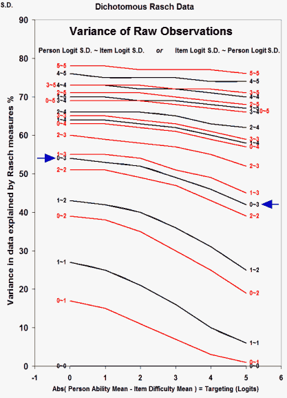
The Figure shows the proportion of raw-observation randomness predicted to exist in dichotomous observations under various conditions.

The x-axis is the absolute difference between the mean of the person and item distributions, from 0 logits to 5 logits. The y-axis is the percent of variance in the data explained by the Rasch measures.

Each plotted line corresponds to one combination of standard deviations. The lesser of the person S.D. and the item S.D. is first, 0 to 5 logits, followed by "~". Then the greater of the person S.D. and the item S.D.

Thus, the arrows indicate the line labeled "0-3". This corresponds to a person S.D. of 0 logits and an item S.D. of 3 logits, or a person S.D. of 0 logits and an item S.D. of 3 logits. The Figure indicates that, with these measure distributions about 50% of the variance in the data is explained by the Rasch measures.

When the person and item S.D.s, are around 1 logit, then only 25% of the variance in the data is explained by the Rasch measures, but when the S.D.s are around 4 logits, then 75% of the variance is explained. Even with very wide person and item distributions with S.D.s of 5 logits only 80% of the variance in the data is explained.

For the unexplained variance, see Critical Eigenvalue Sizes in Standardized Residual Principal Components Analysis (PCA).

In early versions of Winsteps, specify PRCOMP=R

How the Table was computed

This Table was produced with Excel:

1. Normal distributions of logit measures for the items and persons were simulated using specified S.D.s and targeting (= mean difference between person measures and item measures).
2. For each person-item combination were computed:
   the Rasch-dichotomous expected-score: E_ni = 1/(1+exp(D_i-B_n)
   and model-variance of the expected-score: W_ni = E_ni(1-E_ni)
3. The expected scores were averaged
4. Sum-of-squares of explained variance is: sum[(expected score - average expected score)²]
5. Sum-of-squares of unexplained variance is: sum( model-variances of expected scores )
6. Explained variance = (Sum-of-squares of explained variance) / (Sum-of-squares of explained variance + Sum-of-squares of unexplained variance)

Here are some percentages for empirical datasets:

Please email me your own percentages to add to this list.

John Michael Linacre

Editor, Rasch Measurement Transactions

Variance in Data Explained by Rasch Measures. Linacre, J.M. … Rasch Measurement Transactions, 2008, 22:1 p. 1164

The URL of this page is www.rasch.org/rmt/rmt221j.htm

Website: www.rasch.org/rmt/contents.htm